The increase in partisan polarization in the United States over the last several decades is evident in a variety of ways: in roll-call voting in the U.S. Congress1 and state legislatures,2 in voting in state and federal elections,3 in the increased efforts to gain partisan advantage through the drawing of districts for the U.S. House of Representatives and state legislatures,4 in partisan conflict over the appointment of federal judges,5 in patterns of decision-making by the U.S. Supreme Court,6 and patterns of decision-making in federal trial courts.7 But to what degree does the increase in partisanship and polarization appear in judicial elections? The analysis reported in this article shows that partisanship has also increased in statewide elections for state supreme court justices from 1981 to 2020. This increase is particularly striking for nonpartisan elections, but also evident in partisan, semi-partisan, and retention elections.
As of 2021, 39 states use some form of popular election for judicial selection, judicial retention, or both for members of the state’s highest court8 or major trial courts.9 Those elections take one of four general formats: (1) partisan elections in which candidates are listed with their party affiliations on the ballot; (2) semi-partisan elections in which nominations are made either in party primaries or party conventions, but the general election ballot does not identify the political parties that nominated each candidate; (3) nonpartisan elections with no formal role for political parties and no indication on the ballot of the party affiliation, if any, of candidates; and (4) retention elections that use a referendum format asking voters whether the incumbent should be retained for another term.10 One expects partisan elections to produce partisan patterns in voting, and it would not be surprising to find some partisanship in semi-partisan elections. However, a primary goal behind both nonpartisan elections and retention elections is to avoid partisanship, which suggests the voting patterns in those elections should not reflect partisanship.
Research on voting polarization in many types of elections has been traced through survey data. The studies of judicial elections that use survey data to examine the role of partisanship at the individual level are limited because they focus either on a single state11 or on a short period of time.12 Those studies show that partisan patterns do exist in states using both semi-partisan and nonpartisan elections in the years covered. However, there is no body of survey data that would allow the study of changing patterns over time of partisanship in state supreme court elections.
The other approach to studying changing partisanship in state supreme court elections employs aggregate data. In a study of state supreme court elections between 1946 and 2012, I used county data to examine partisan patterns in all four types of state supreme court elections conducted on a statewide basis.13 Specifically, I computed the correlation between the county-level voting percentages supporting the Democratic candidate for governor and the voting percentages supporting one of the candidates for state supreme court or, in states using retention elections, the percentage favoring a judge’s retention. I labeled the resulting correlations, which can range from -1 to +1, “partisan correlations.”14 That analysis showed evidence that partisanship had increased in some of the states using the very types of elections — nonpartisan and retention elections — that were intended to avoid partisanship.15
Since 2012, partisan polarization in the United States has continued to increase. This is evident in several state supreme court elections, using three of the election formats, held in 2020. In Wisconsin, a state that uses nonpartisan elections for judicial positions (and until about 25 years ago had a strong tradition of nonpartisanship16), liberal challenger Jill Karofsky defeated conservative incumbent Daniel Kelly, whom Republican Governor Scott Walker had appointed in 2016 to fill a vacancy caused by the retirement of conservative justice David Prosser.17 Karofsky won with 55.3 percent of the vote. More important was the very strong partisan pattern, evident in both county-level and ward-level voting returns: The correlation between the percentage of voters who supported Karofsky and the percentage voting for Democrat Tony Evers in the 2018 gubernatorial election exceeded .9 both at the county level and at the ward level (.96 at the county level, and .91 at the ward level). That is, at the county (or ward) level, knowing the percentage of voters who voted for the Democratic candidate in each county (or ward) in Wisconsin’s partisan gubernatorial election explains 96 percent of the variation across counties in the percent voting for the liberal candidate in the nonpartisan judicial election. The county-level correlation in Wisconsin’s nonpartisan format was only slightly below the average county-level correlation for elections in states with partisan supreme court elections in 2020 (.98), and was above the average correlation for elections in states with semi-partisan supreme court elections (.87).
Even the partisan elections have been getting more partisan. The average county-level correlation between partisan state supreme court elections and the most recent gubernatorial elections in 2020 was higher than that of all but two other election cycles since 1946. North Carolina, which had three supreme court elections in 2020, produced county-level correlations of .993, .994, and .993; the precinct-level correlations were .997, .997, and .993. In fact, except for one Oklahoma election in 1946 and five North Carolina elections between 1948 and 1952, all of the partisan elections with county-level correlations exceeding .99 occurred in 2018 or 2020.
Since 1936, there have been 855 retention elections for state supreme courts,18 but only 13 justices seeking retention have been defeated. One of those defeats came in 2020 with Illinois Supreme Court Justice Tom Kilbride losing his retention bid; a solid majority of voters favored retention (56.5 percent), but Kilbride failed to get the 60 percent required for retention in Illinois.19 Republicans mounted a concerted campaign against Kilbride, with extensive television advertising funded by conservative interests that linked Kilbride to the Democratic Speaker of the Illinois State House of Representatives.20 The correlation between the vote for the Democratic candidate for governor in 2018 and for retaining Justice Kilbride was .50 when using the 22 counties in Kilbride’s district as units;21 across 1,393 precincts in those counties, the correlation was .72.22
Importantly, the correlations in the Kilbride retention election were not exceptional. The highest county-level correlation for a 2020 retention election was .91 in Justice Melissa Hart’s election in Colorado; Justice Hart was easily retained with almost 75 percent voting in favor of her retention. This was not surprising given that she was unanimously recommended for retention by the Colorado Office of Judicial Performance Evaluation,23 as was the other Colorado Supreme Court justice, Carlos Samour, who also easily won retention in the same election (and for whom the partisan correlation was .89).24 This high correlation occurred even as a majority of voters in every county favored retaining both Justice Hart and Justice Samour, with majorities ranging from 52.1 percent to 87.2 percent for Hart and from 51.5 percent to 84.4 percent for Samour.25
In the balance of this article, I first explain the idea of the “partisan correlation” and then provide more detailed evidence of the increasing partisanship in statewide state supreme court elections. That analysis will show that in each decade since 1971, partisan polarization has increased in all four types of elections but not in every state using statewide elections for the state’s supreme court.
The idea of correlating county-level results in state supreme court elections with results for gubernatorial elections goes back 50 years to Kathleen Barber’s 1971 study of Ohio’s Supreme Court elections.26 Her approach was extended to several other states by David Adamany and Philip Dubois,27 and then to many more states by Philip Dubois.28 The 2020 election in Wisconsin, a state using nonpartisan elections held at a different time (April) than the November partisan elections, is a good example of the relationship between voting in state supreme court election and voting in the gubernatorial election. The top graph in Figure 1 (below) shows a county-level plot of the 2020 percentage of votes for Jill Karofsky against percentage of the two-party vote (i.e., ignoring third parties) received by Democratic gubernatorial candidate Tony Evers in the 2018 partisan gubernatorial election; each dot in the plot represents one of the 72 Wisconsin counties, and the straight line is the best fit line showing the relationship between those two sets of votes. The high correlation noted previously reflects that almost all of the dots are tightly clustered around the line. The pattern in elections with lower correlations would have the dots more scattered around the line, and if the correlation was zero, the line would be perfectly horizontal.

The advantage of using county-level results is that the data are relatively available compared to smaller units such as precincts or wards.29 Although one might expect that correlations would increase as the degree of aggregation increased, that does not appear to necessarily be the case; sometimes the correlation is higher (Wisconsin 2020) with counties compared to smaller units, and sometimes it is lower (Illinos 2020). For the 2020 Wisconsin Supreme Court election, the correlation using ward-level data is slightly lower, and the bottom graph in Figure 1 shows why that is the case: Although most points cluster tightly around the line, there are more dots farther off the line. Even if data were readily available at the precinct or ward level, there would be potential problems created by the lack of stability of the boundaries or names of these smaller units (wards and precincts). In matching the 2018 and 2020 data for Wisconsin, many wards did not match between the two elections and could not be used in computing the correlation. In contrast, counties — both in geographic boundaries and names — are very stable in the contemporary United States.
There are several complications with the computation of partisan correlations that should be noted. First, how to handle judicial elections not occurring in the same year as a gubernatorial election? The approach used here is to average county-level percentages of the two adjacent gubernatorial elections and compute the correlation using those averages.30 For judicial elections in 2019 and 2020 in states where the last gubernatorial election was in 2018, the 2018 gubernatorial election results were used. Second, how to handle third-party candidates, either in the gubernatorial election or the judicial election? Those candidates were ignored in computing percentages, meaning that all percentages used were the two-party results. Third, how to handle nonpartisan elections? I made no attempt to link judicial candidates to parties in nonpartisan elections,31 and the absolute value of the correlation between the election and the gubernatorial election was used.32 Finally, how to compute correlations in multi-seat elections in which n seats are to be filled, voters could cast votes for n candidates, and the n candidates with the most votes win? In those elections, correlations were computed by matching the top vote-getter with the bottom vote-getter, second from the top with second from the bottom, and, if necessary, the third from the top with the third from the bottom.
Computing the partisan correlation for yes-no retention elections involves the complication that there is no party in the context of those elections. If one computes the correlation between the percent voting for the Democratic candidate for governor and the percent voting in favor of retention, that correlation can be either positive (the line slopes up) or negative (the line slopes down). My interest here is the magnitude of the correlation, and so it is the absolute value of the correlation that is important; however, in some graphs, I use different colors and symbols to indicate whether the favorable vote increased with the Democratic vote share for governor (shown in blue circles) or decreased — i.e., increased with the Republican vote share (shown in red Xs; see Figure 8 on page 72).33
County-level data for state supreme court elections used in the analysis presented here come from an archive I created, which is available on the Harvard Dataverse.34 The data cover elections from 1945 to 2020 and were assembled from online reports by state offices, published reports, and in a few instances unpublished materials obtained from state archives. The sub-county data referenced earlier were obtained from official state websites in the relevant states. A small number of states hold judicial elections in odd-numbered years; many of the results that follow group those elections into a two-year election cycle, combining them with the elections in the following even-numbered year.
Broad Patterns
Figure 2 provides a quick snapshot of patterns for the average partisan correlation by decade for the four elections types. The figure shows that the average partisan correlation started increasing in all four types of elections after the 1971–1980 decade, either after a decline (in partisan and retention elections) or a mixed pattern of variation (in semi-partisan and nonpartisan elections). Clearly, partisanship has increased over the last 40 years, but perhaps more interesting is the increase in the proportion of partisan correlations exceeding .9. Figure 3 shows the percentage of partisan correlations across all election types in four bands — less than .6, .6 – <.8, .8 – <.9, and .9 or greater — for each two-year election cycle since 1946. The figure shows a pattern of a decreasing percentage of elections with a partisan correlation exceeding .9 until the 1980s, when that percentage began to increase such that the percentage in the most recent election cycle (2020, at 35.2 percent) exceeds that in the earliest cycle shown (1946, at 31.7 percent) as well as all other cycles shown in the figure.
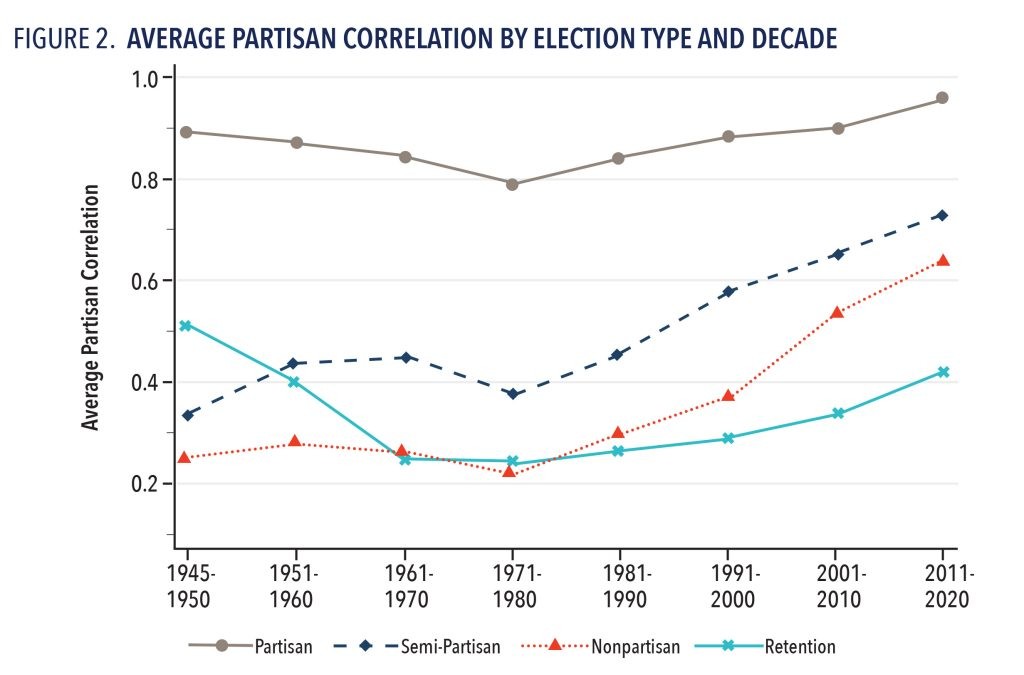

This increase is more striking given the way the types of elections used in these states changed over a 75-year period. For example, prior to 1960, only California and Missouri used retention elections; by 2020, 17 states used retention elections for supreme court elections.35 More importantly, the number of states using partisan elections dropped from 14 to six.36 Figure 4 (next page) shows the change in the percentage of supreme court elections by type. In the two earliest decades, partisan elections constituted almost 60 percent of these elections; that number dropped to under 20 percent in the last two decades. At the same time, retention elections increased from about 4 percent to about 40 percent of statewide supreme court elections. Before 2002, only two elections had partisan correlations exceeding .9 that were not partisan elections; those were 1986 retention elections for California Supreme Court Justices Rose Bird and Cruz Reynoso, both of whom were defeated.37 So, even as the partisan election format fell out of favor nationally, partisanship in those elections rose.

Partisan Elections
Figure 5 shows that the partisan correlations for statewide partisan elections increased modestly starting around 1988.38 I start with the 1981–1982 election cycle because half of the 18 states using statewide partisan elections in 1945 had ceased doing so by 1980. The figure omits a small number of elections in Georgia (which switched to nonpartisan elections in 1984) and in Tennessee (which switched to a Missouri Plan system — a format in which governors appoint from a list of nominees prepared by a nominating commission, and sitting justices stand in retention elections at the end of their current terms — in 1994). The figure includes Arkansas (which switched to nonpartisan elections in 2002), West Virginia (which switched to nonpartisan elections in 2016), and North Carolina (which switched to nonpartisan elections in 2004 but reinstated partisan elections in 2018).

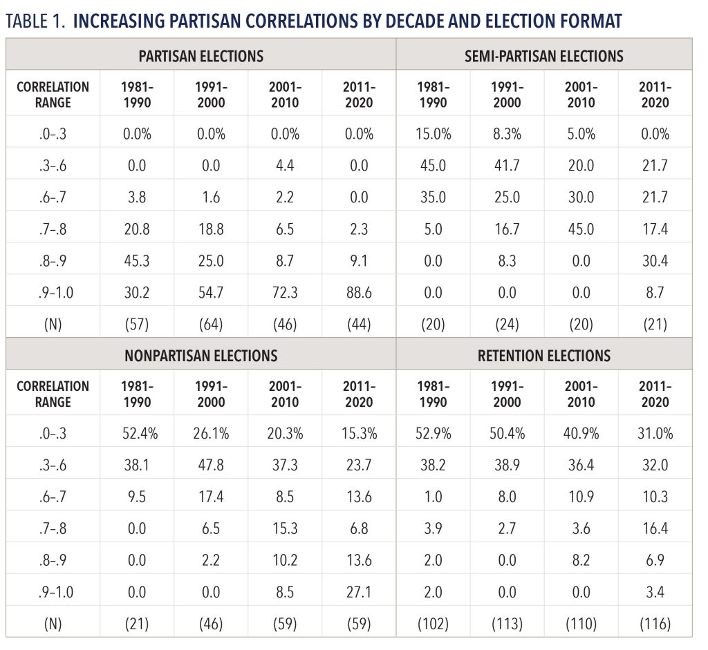
The line, fitted using the LOWESS procedure,39 makes it clear that partisan correlations started increasing in the late 1980s. The percentages listed across the bottom of the figure represent elections not contested by both parties, although many of those elections were contested in party primaries or by third parties. Not surprisingly, a majority (60.1 percent) of these elections produced partisan correlations exceeding .9, and only two elections produced correlations below .6. The figure shows that the correlations are increasingly clustered toward the top of the possible range over the 40-year period shown. As indicated in Table 1, from 1981 to 1990 only 30.2 percent of the correlations exceeded .9. That percentage increased over the three succeeding decades: 54.7 percent for 1991–2000, 78.3 percent for 2001–2010, and 88.6 percent for 2011–2020. For the last decade, no elections produced a partisan correlation below .7. Thus, even in the type of elections in which one would expect strong partisan patterns, partisanship has increased significantly over the last 40 years.
Semi-Partisan Elections
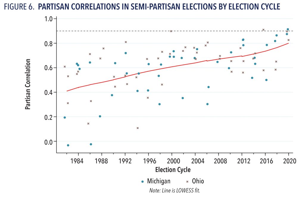
As of 2020, only two states, Ohio and Michigan, used systems in which parties make nominations but party labels are not included on the general election ballot.40 Nominations are made by party primaries in Ohio and by state party conventions in Michigan.41 Although Figure 2 shows an increase in the average partisan correlation starting after the 1971–1980 decade, the average for that decade was low compared to the prior decades. The average for 1981–1990 returned to the level of the three periods prior to 1971–1980. Because the analysis here covers the period 1981 through 2020, it does not include five elections that produced much higher negative correlations: -.42 in a 1970 Ohio election and four elections in Michigan (1949, 1956, 1968, and 1976) in which the negative correlation ranged from -.20 to -.26.
Figure 6 shows the pattern of partisan correlations for Ohio and Michigan. The correlations are shown in turquoise circles for Michigan and brown Xs for Ohio. The LOWESS line shows the increase over the period. Only four of the 93 elections during this period were uncontested.42 As one would expect, correlations cover a wide range, and extreme correlations are rare. However, while correlations exceeded .8 just twice prior to 2000, there have been 10 correlations of .8 or greater since then. And since 2016, the correlation has twice exceeded .9 — once in an Ohio election and once in a Michigan election. Mid-range correlations between .6 and .8 have increased sharply, as shown in Table 1, and in the last decade no correlations were below .3. Thus, even without partisan labels on the ballot, partisan voting has greatly increased in these semi-partisan election states.
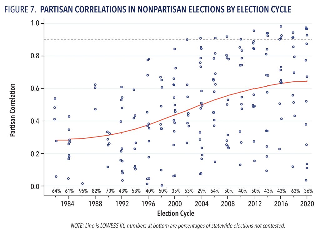
Nonpartisan Elections
As shown in Figure 2, nonpartisan elections have, overall, seen the sharpest increase in partisan correlations.43 Figure 7 shows the absolute partisan correlations for all statewide nonpartisan elections between the 1981–1982 election cycle and the 2019–2020 cycle. As with Figure 5, the numbers across the bottom are the percentages of statewide nonpartisan elections that were uncontested in each election cycle. The LOWESS line shows that the partisan correlations were increasing over the entire period, but the greatest rate of increase occurred between the 1991–1992 and the 2009–2010 cycles. Table 1 shows that, during the first decade, the majority (52.4 percent) of the correlations were less than .3. Only 9.5 percent of the correlations exceeded .6, and none exceeded .7. The first correlations exceeding .8 appeared in the second decade, which is also when an increasing proportion of the correlations exceeded .6. Starting around 2000, correlations exceeding .8 were increasingly frequent, exceeding 40 percent in the 2011–2020 decade (27.1 percent exceeded .9.) By the last decade, only 20.3 percent of the correlations were less than .3.
A state-by-state analysis using statewide nonpartisan elections since 1981 (see Figure A3 in the Appendix online at judicature.duke.edu/partisancorrelation) shows that only one state, Oregon, had an election with a partisan correlation exceeding .6 in the 1981–1990 decade. During that decade, the partisan correlation was under .3 in most elections. But by 1991–2000, Oregon had broken the .8 barrier. In the 2001–2010 decade, Washington had five elections in which the partisan correlation exceeded .9; one or more elections in North Carolina,44 Oregon, and Wisconsin had correlations exceeding .8, and 41.0 percent of all contested elections had partisan correlations exceeding .6. In the most recent decade, five states had one or more elections with correlations greater than .9, and 59.0 percent of the correlations exceeded .6. The only states with no partisan correlations exceeding .6 during the most recent decade are Arkansas and North Dakota. Thus, the degree of polarization varies among the states but has been strongest in North Carolina, Washington, Wisconsin, and possibly Oregon. However, one must keep in mind that in some states, including Oregon and Washington, a significant proportion of elections were uncontested (as shown by the numbers in the row just above the state abbreviations in Figure A3 in the Appendix online at judicature.duke.edu/partisancorrelation).
Retention Elections
Figure 8 shows that absolute partisan correlations in statewide retention elections between 1981 and 2020 have increased, but more modestly than for semi-partisan and nonpartisan elections. The blue circles in the figure represent positive correlations, indicating that the support for retention increased as the support for the Democratic gubernatorial candidate increased.
The red Xs represent negative correlations, indicating that support for retention increased as support for the Republican gubernatorial candidate increased. The LOWESS line shows a slight tendency for the correlation to decrease through the 1980s before starting a gradual increase in the 1990s. The three blue circles just above and below .9 in 1986 are from the California election; the blue circle just below .9 in 1982 is also from California. It took almost 30 years for the correlation to again exceed .9. Table 1 makes clear that there was an increase in the absolute partisan correlations in retention elections. In the 1981–1990 decade, 52.9 percent of the correlations were under .3, and 91.1 percent were under .6. In the 2011–2020, decade, these percentages dropped to 21.0 and 63.0, respectively, as the correlations over .6 increased from 8.9 percent in 1981-1990 to 37 percent in 2011-2020. The increase is not as great as in nonpartisan elections, but it is nonetheless substantial.
A state-by-state analysis (see Figure A4 in the Appendix online at judicature.duke.edu/partisancorrelation) also shows that absolute partisan correlations vary quite a bit among the states
using retention elections. The only state besides California where one or more partisan correlations exceeded .9 was Colorado in Justice Hart’s 2020 retention election.45 Moreover, only a few additional states had any correlations exceeding .8: Alaska (1982, 2010, 2016, and 2020),46 Iowa (2010), New Mexico (2006), and South Dakota (2020).47
Given the controversy over the Iowa Supreme Court’s 2009 same-sex marriage decision and the campaign against the three justices standing for retention in 2010,48 the state’s strong partisan correlations (all three correlations were .84) that year were not surprising. Although organized campaigns opposing retention will usually boost the magnitude of partisan correlations, the example of the 2020 retention elections in Colorado and South Dakota show that strong correlations can happen even in the absence of such campaigns.49 In the other state with a correlation exceeding .8 in 2020, Alaska Supreme Court Justice Susan M. Carney faced organized opposition from conservative groups focused on decisions related to sexual offender registration and abortion.50 Primarily, though, analysis shows that partisan correlations vary substantially among the states using retention elections. (See Figure A4 in the Appendix online at judicature.duke.edu/partisancorrelation.)
Clearly, partisanship has increased in all four forms of judicial elections during recent decades, although the degree of increase and the degree of change varies across and within the election types. The sharpest increase has been in nonpartisan elections, but the increase in semi-partisan elections is only slightly lower. The magnitude of the increase in partisan elections is much lower, but that is in part because the typical correlation was already close to the limiting value of 1. However, if one applies a standard transformation to the correlation values, that relaxes the limiting effect, and the transformed version of the correlation for partisan elections more than doubles over the 40-year period.51 Though the increase in absolute partisan correlations in retention elections is more modest than the other election types, it is still clearly observable.
Is it possible that these changes result from changes in other measurable factors? One could argue that three broad political changes during this 40-year period explain the increasing partisanship in judicial elections: changes in the party competitiveness of the states, changes in the degree of partisan polarization in the states, and increasing use of attack advertising,52 particularly television advertising. I explored each of these as possible explanations for the increased partisanship in state supreme court elections. Using two different measures of state-level party competitiveness — low competitiveness is when one party dominates in state-level politics and high competitiveness is when neither party dominates53 — I found that both tended to predict, to varying degrees, the partisan correlation in state supreme court elections. One surprising result was that the relationships varied with the type of election format; each of the two measures predicted the correlation for only one type of election. Also, surprisingly, the partisan correlation tended to increase as party competitiveness decreased; this probably means that the presence of a dominant party (low party competitiveness) leads to more stable patterns in the judicial elections across counties, increasing the partisan correlation. Using a measure of partisan polarization based on roll call voting in state legislatures,54 I found the clearest relationship was for retention elections; the increased absolute partisan correlation was largely accounted for by the measure of legislative polarization. There was a lesser effect for partisan elections and no effect for nonpartisan or semi-partisan elections. Information on television advertising is only available starting in 1999; 55 I found no relationship between the presence of televised attack advertisements in a state supreme court election and the partisan correlation. Perhaps the most interesting of these results is the absence of a relationship between legislative polarization and the partisan correlation in nonpartisan elections, the type of elections that had the most striking increase in partisan correlations.
Judicial elections, at least those for state supreme courts, have not escaped the increasing partisanship associated with political polarization. This is especially true for those election formats that were designed to avoid partisanship, at least in some states. Some of this increased partisanship in states with nonpartisan and retention elections relates to court decisions in politically salient policy areas. The strong partisan pattern in the 2010 Iowa retention election was almost certainly a response to the Iowa Supreme Court’s same-sex marriage decision. Similar examples can be found in states with nonpartisan elections such as Wisconsin and Washington, among others.
An important question is whether there is causation in the other direction: Does increased partisanship in state supreme court elections lead to increased polarization on state supreme courts? One can easily find anecdotal evidence that would support such a conclusion (e.g., in Wisconsin), but a more systematic analysis would require time-series data on state supreme court decisions along with a specification of which types of cases one would expect to show increased polarization. Modern systems of automated text analysis may make it possible to develop the needed data in the near-term, but until then a systematic analysis of the impact of increased partisanship on state supreme courts remains to be addressed by future research.
Finally, given the increased political polarization over the last two or three decades, it should not be surprising that judicial elections are increasingly partisan. That increase is strongest in nonpartisan elections, probably because nonpartisan elections had such low levels of partisan correlations to begin with compared to partisan and semi-partisan elections. That the increase in partisanship in retention elections has remained (again, relatively) low for most of those elections almost certainly reflects the fact that, unlike nonpartisan elections with two or more candidates competing for votes, most retention elections have remained largely out of sight of the voters.
